The problem of statistical data processing in ultrasonic pile testing
Statistical data processing in ultrasonic testing of pile concrete is a real challenge for testing laboratories. MIT UZK MONOLITH from M-Instrument has solved this problem. GOST R 71039-2023 recommends computing the mean (normal) velocity on the measurement profile using a statistical data-processing algorithm that applies robust estimation methods. Yet the Russian standard contains no calculation or analysis algorithm, leaving this complex and critical data-processing task to the discretion of the operator.
We decided to review foreign standards. The results of analyzing foreign technical codes formed the basis of the MIT UZK MONOLITH statistical processing algorithm.
Review of foreign standards: USA, France, China
ASTM D6760-16 (USA) and NF P 94-160-1 (France) do not provide statistical methods. Integrity is assessed through visual analysis of the time and energy transmission plots of the ultrasonic signal. These standards set only minimum requirements and rely on the qualification of the specialist, who determines the presence of a defect.
JGJ 106-2014 (China) contains a probabilistic-statistical evaluation method. It consists of iteratively discarding extreme velocity values while computing the mean, standard deviation, and critical values for the remaining sample. It is precisely this data-processing algorithm that forms the basis of MIT UZK MONOLITH. We examine this algorithm in detail below.

Statistical data processing algorithm implemented in MIT UZK MONOLITH
1. Calculation of time, velocity, amplitude and frequency for each acoustic line
In parallel or inclined scanning, the values of time, sound velocity, amplitude and wave frequency for each acoustic line are calculated from on-site test data according to the following formulas:
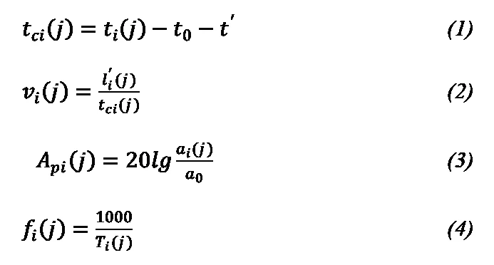
where
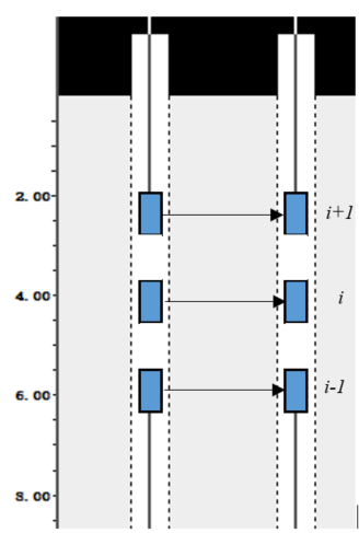
- i — the number of the acoustic line, assigned sequentially from bottom to top (or top to bottom) for each measurement profile;
- j — the number of the measurement profile;
- time of the i-th acoustic line of the j-th measurement profile, μs;
- measured value of the acoustic time of the i-th acoustic line of the j-th measurement profile, μs;
- instrument delay, μs;
- time correction for acoustic tubes and the water coupling layer, μs;
- distance between the outer walls of two acoustic tubes along the i-th acoustic line of the j-th measurement profile, mm. With parallel tube arrangement it is acceptable to take the distance between the outer walls of the tubes at the pile head level; with inclined scanning it is the distance between the outer walls of the tubes at points corresponding to the mid-points of the transmitting and receiving transducers, which can be derived from the distance between the tubes at the pile head and the difference in transducer elevations;
- sound velocity of the i-th acoustic line of the j-th measurement profile, km/s;
- first-arrival amplitude of the wave of the i-th acoustic line of the j-th measurement profile, dB;
- first-arrival amplitude of the signal of the i-th acoustic line of the j-th measurement profile, V;
- signal amplitude corresponding to zero decibels, V;
- signal frequency of the i-th acoustic line of the j-th measurement profile, kHz, obtainable by spectral analysis of the signal;
- signal period of the i-th acoustic line of the j-th measurement profile (μs).
2. Probabilistic statistical values for identifying velocity anomalies
When using parallel or inclined scanning, the probabilistic statistical values for identifying sound velocity anomalies for the j-th measurement profile are determined by the following procedure:
2.1. Arrange the sound velocity values of each acoustic line of the j-th measurement profile in descending order and sequentially apply the formula: (4)
where
- sound velocity of the i-th acoustic line of the j-th measurement profile, i = 1, 2, …, n;
- n — total number of acoustic lines in the j-th measurement profile;
- k — number of smallest sound velocity values to be removed, k = 0, 1, 2, …;
- k' — number of largest sound velocity values to be removed, k' = 0, 1, 2, ….
2.2. For the data remaining after the sequential removal of k smallest and k' largest values, statistical calculations are performed using the following formulas: (5), (6), (7), (8), (9)
where
- estimated anomaly value for small readings;
- estimated anomaly value for large readings;
- mean value;
- standard deviation;
- coefficient of variation;
- λ — coefficient (outlier detection criterion) determined from Table 1 depending on (n - k - k').
Note: the λ coefficient is used to determine the normal-range bounds depending on the size of the sample of individual measurement results.
Table 1. Values of the statistical coefficient λ for probabilistic identification of sound velocity anomalies
| n | 10 | 11 | 12 | 13 | 14 | 15 | 16 | 17 | 18 | 20 |
|---|---|---|---|---|---|---|---|---|---|---|
| λ | 1.28 | 1.33 | 1.38 | 1.43 | 1.47 | 1.50 | 1.53 | 1.56 | 1.59 | 1.64 |
| n | 20 | 22 | 24 | 26 | 28 | 30 | 32 | 34 | 36 | 38 |
| λ | 1.64 | 1.69 | 1.73 | 1.77 | 1.80 | 1.83 | 1.86 | 1.89 | 1.91 | 1.94 |
| n | 40 | 42 | 44 | 46 | 48 | 50 | 52 | 54 | 56 | 58 |
| λ | 1.96 | 1.98 | 2.00 | 2.02 | 2.04 | 2.05 | 2.07 | 2.09 | 2.10 | 2.11 |
| n | 60 | 62 | 64 | 66 | 68 | 70 | 72 | 74 | 76 | 78 |
| λ | 2.13 | 2.14 | 2.15 | 2.17 | 2.18 | 2.19 | 2.20 | 2.21 | 2.22 | 2.23 |
| n | 80 | 82 | 84 | 86 | 88 | 90 | 92 | 94 | 96 | 98 |
| λ | 2.24 | 2.25 | 2.26 | 2.27 | 2.28 | 2.29 | 2.29 | 2.30 | 2.31 | 2.32 |
| n | 100 | 105 | 110 | 115 | 120 | 125 | 130 | 135 | 140 | 145 |
| λ | 2.33 | 2.34 | 2.36 | 2.38 | 2.39 | 2.41 | 2.42 | 2.43 | 2.45 | 2.46 |
| n | 150 | 160 | 170 | 180 | 190 | 200 | 220 | 240 | 260 | 280 |
| λ | 2.47 | 2.50 | 2.52 | 2.54 | 2.56 | 2.58 | 2.61 | 2.64 | 2.67 | 2.69 |
| n | 300 | 320 | 340 | 360 | 380 | 400 | 420 | 440 | 470 | 500 |
| λ | 2.72 | 2.74 | 2.76 | 2.77 | 2.79 | 2.81 | 2.82 | 2.84 | 2.86 | 2.88 |
| n | 550 | 600 | 650 | 700 | 750 | 800 | 850 | 900 | 950 | 1000 |
| λ | 2.91 | 2.94 | 2.96 | 2.98 | 3.00 | 3.02 | 3.04 | 3.06 | 3.08 | 3.09 |
| n | 1100 | 1200 | 1300 | 1400 | 1500 | 1600 | 1700 | 1800 | 1900 | 2000 |
| λ | 3.12 | 3.14 | 3.17 | 3.19 | 3.21 | 3.23 | 3.24 | 3.26 | 3.28 | 3.29 |
2.3. In the order k = 0, k' = 0; k = 1, k' = 1; k = 2, k' = 2 … the smallest value in the statistical sample is sequentially compared with the estimated anomaly value for small readings. When the condition is met, the smallest value is removed. The largest value is compared with the estimated anomaly value for large readings. When the condition is met, the largest value is removed. Only one value is removed at a time; the calculation steps are repeated for the remaining data sequence until both of the following conditions are met: (10), (11)
3. Critical value for identifying sound velocity anomalies
The probabilistic statistical value for identifying sound velocity anomalies for the j-th measurement profile is computed by the formula: (12)
where this is the probabilistic statistical value for identifying sound velocity anomalies of the j-th measurement profile.
For a pile with only one measurement profile, its critical value for identifying sound velocity anomalies equals the critical value for identifying sound velocity anomalies on that measurement profile, i.e.: (13)
For a pile with three or more measurement profiles, the critical value for identifying sound velocity anomalies for each acoustic line of the pile is taken as the arithmetic mean of the critical values for identifying sound velocity anomalies of each measurement profile, i.e.: (14)
where
- critical value for identifying sound velocity anomalies on the j-th measurement profile;
- probabilistic statistical value for identifying sound velocity anomalies on the j-th measurement profile.
4. Identification of a sound velocity anomaly
A sound velocity anomaly is identified from the following condition: (15)
where
- sound velocity of the i-th acoustic line of the j-th measurement profile;
- critical value for identifying sound velocity anomalies of the j-th measurement profile.
5. Critical value for identifying wave amplitude anomalies
The critical value for identifying wave amplitude anomalies is computed by the following formulas: (16), (17)
An amplitude value is considered anomalous if the following condition is met: (18)
where
- mean amplitude value of all acoustic lines of the j-th measurement profile (dB);
- amplitude value of the i-th acoustic line of the j-th measurement profile (dB);
- critical value for identifying wave amplitude anomalies of the j-th measurement profile (dB);
- n — total number of acoustic lines in the j-th measurement profile.
6. PSD criterion (Probability Slope Difference; slope method)
The PSD criterion is used as an auxiliary criterion for identifying anomalous acoustic lines. The PSD value is the product of the slope of the line connecting two adjacent points on the time–depth curve and the difference of time values, and is computed by the following formula: (20)
where
- PSD — PSD value, μs²/m;
- acoustic time of the i-th acoustic line of the j-th measurement profile, μs;
- acoustic time of the (i-1)-th acoustic line of the j-th measurement profile, μs;
- depth of the i-th acoustic line, m;
- depth of the (i-1)-th acoustic line, m.
Note: if the PSD value undergoes an abrupt change (a jump) at a given depth, it is recommended to analyze the PSD criterion together with wave amplitude changes.
Algorithm results in the MIT UZK MONOLITH software suite
Based on calculations using the algorithm above, the MIT UZK MONOLITH software suite presents the user with a measurement results table (see Fig. 3). Ultrasonic velocity and signal amplitude values that fail the assessment criteria are highlighted in red font:
- actual velocity at the measurement point is below the critical value;
- actual signal amplitude is more than 6 dB below the mean.
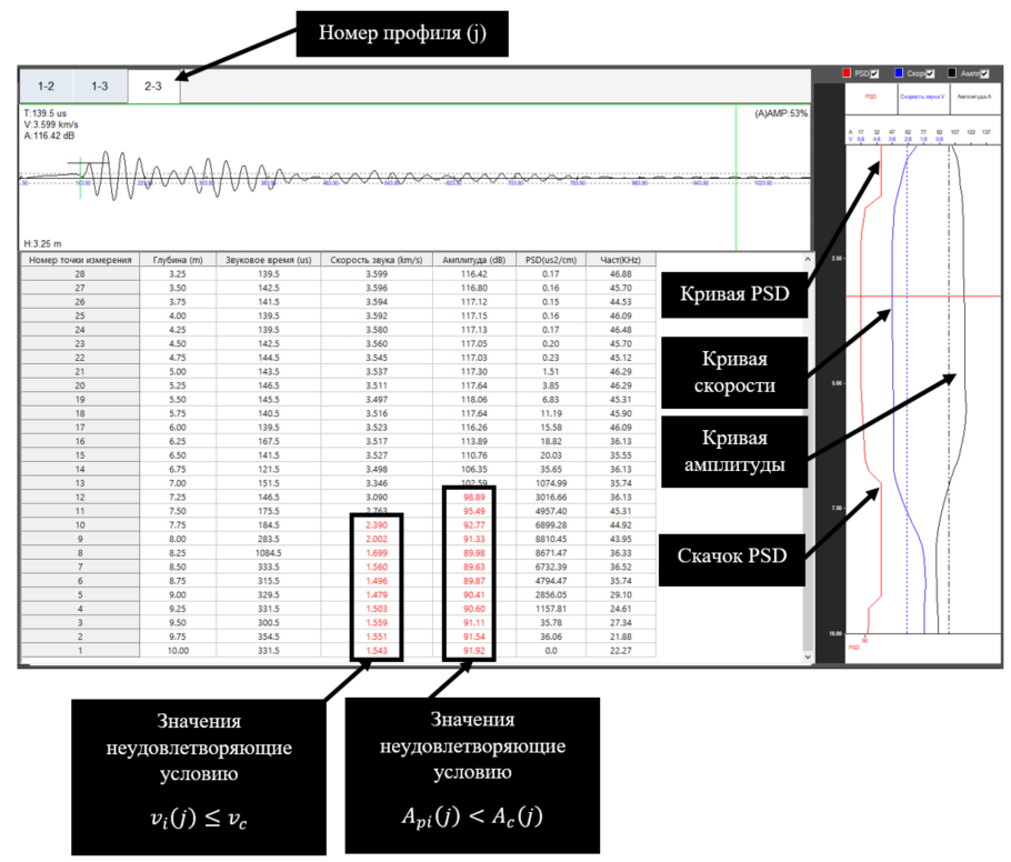
Use of the MIT UZK Monolith 1-2k instrument together with the MIT UZK MONOLITH software suite solves the problem of statistical data processing in ultrasonic integrity testing of pile concrete.
Video: working with the instrument and the software suite
You can learn about working with the MIT UZK Monolith 1-2k instrument in this video:

More on working with the MIT UZK MONOLITH software suite:

References
- GOST R 71039-2023. Bored piles and trench- and pile-type diaphragm walls. Crosshole ultrasonic method for concrete quality testing.
- ASTM D6760-16. Standard Test Method for Integrity Testing of Concrete Deep Foundations by Ultrasonic Crosshole Testing.
- NF P 94-160-1. Soils: investigation and testing — auscultation of a foundation — Part 1: Sonic coring (acoustic logging).
- JGJ 106-2014. Technical code for testing of building foundation piles.
Want to use this algorithm in your own laboratory?
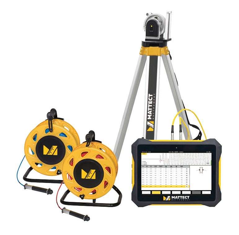
MIT UZK Monolith 1-2k is a two-channel instrument for pile UT per GOST R 71039-2023 with automatic statistical processing
Frequently asked questions
Why does MIT UZK MONOLITH use the Chinese JGJ 106-2014 rather than Russian GOST R 71039-2023?
Russian GOST R 71039-2023 recommends the use of robust estimation methods but does not provide specific calculation formulas. We studied ASTM D6760 (USA), NF P 94-160-1 (France) and JGJ 106-2014 (China). Only JGJ 106-2014 contains a complete probabilistic-statistical algorithm with iterative removal of extreme values — which is what we implemented in MIT UZK MONOLITH.
How does the MIT UZK MONOLITH algorithm reject anomalous ultrasonic velocity values?
Velocity values for each acoustic line are sorted in descending order. Then the mean, standard deviation, coefficient of variation, and anomaly estimation values for low and high readings are computed sequentially. Each smallest and largest value is compared with the outlier criteria; if the condition is met, it is removed. The procedure is repeated until both extreme values fall within the acceptable range.
What is the PSD criterion and when is it applied?
PSD (Probability Slope Difference — the slope method) is an auxiliary criterion for identifying anomalous acoustic lines. The PSD value is the product of the slope of the line connecting two adjacent points on the time–depth curve and the difference of time values. Sharp jumps in PSD at a given depth signal a possible defect — in that case the analysis is combined with wave amplitude changes.
Is the MIT UZK MONOLITH algorithm compatible with ASTM D6760?
ASTM D6760-16 and the French NF P 94-160-1 do not contain statistical evaluation methods — they establish minimum requirements and rely on operator qualification, with the operator determining the presence of a defect. The JGJ 106-2014 algorithm in MIT UZK MONOLITH goes further — it automates statistical processing and removes subjectivity from the assessment, which satisfies both the spirit of ASTM D6760 and the requirements of GOST R 71039-2023 for robust methods.
How does MIT UZK MONOLITH present statistical processing results?
The MIT UZK MONOLITH software suite builds a measurement results table with automatic red-font highlighting of values that fail the assessment criteria: actual ultrasonic velocity below the critical value, or actual signal amplitude more than 6 dB below the mean. The operator immediately sees problem acoustic lines and depths.
Author: Denis Vorobev, Chief Laboratory Manager at MATTEST LLC. Expert content prepared for the website of partner company M-Instrument LLC (MATTEST INSTRUMENT).