
In the previous article, we examined the main tools for processing a signal in the time domain and discussed the signal processing workflow for obtaining a waveform of the required shape.
In this article, we will examine the frequency domain of a seismoacoustic signal and explain how it works.
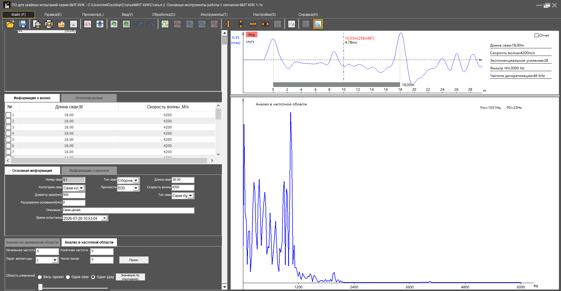
Fig. 1. Screen view when working with a signal in the frequency domain.
In the author’s opinion, signal processing in the frequency domain is already an advanced skill in seismoacoustics.
Whereas in the “Time-domain analysis” section we worked with a waveform (a time/depth signal), the “Frequency-domain processing” section involves moving to the signal spectrum (the signal by frequency).
The instrument applies the Fourier transform: it automatically decomposes a complex signal into individual frequencies and displays them as an Amplitude/Frequency graph.
Frequency-domain analysis does not replace time-domain analysis; it complements it. First, the time/depth waveform must be analysed to identify suspicious areas. Only then should you switch to frequency-domain analysis to confirm or rule out possible suspicions of a defect.
The following tools are available for frequency-domain work: start and end frequency, number of peaks, and amplitude threshold.

Fig. 2. Tools for processing a signal in the frequency domain.
Start/end frequency: the frequency at which the search for peaks on the graph starts/ends (in Hz);
Number of peaks: the number of peaks to be found;
Amplitude threshold: the minimum amplitude at which a peak is taken into account. Peaks with amplitudes below this threshold are not included in the search results;
Search: pressing the “Search” button starts the peak search procedure, after which the intervals between adjacent peaks are displayed.
In general, there are some basic points worth considering:
The physics of a seismoacoustic signal passing through pile concrete is as follows: solid (defect-free) concrete transmits low frequencies, while defects “absorb the lows” and amplify the highs.
Analysis of the “low/high” ratio.
Pay attention to which frequency has become more prevalent after the wave has passed through. If the signal has lost low frequencies (the frequency values have shifted upwards), this indicates an abrupt change in cross-section (a narrowing or a void).
Distinguishing a defect from a contrasting geological boundary.
On the waveform, both a defect and an interface between soils produce reflections. In the frequency domain, a reflection from a soil boundary produces low frequencies, whereas a reflection from a defect shifts the spectrum upwards.
Blind zones.
Sometimes a reflection from a defect merges with the initial pulse (within 1–2 m of the pile head). In the frequency domain, these zones are visible through changes in spectral composition even without a clear peak on the graph.
Let us consider several examples.
Example 1.
We will specify the frequency range of interest and the number of peaks, then interpret the results obtained for a defect-free pile.
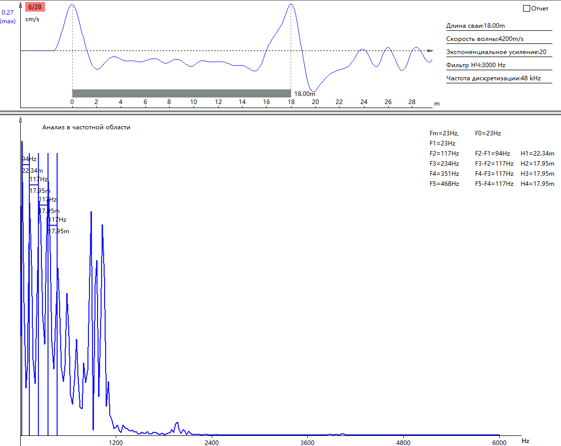
Fig. 3. Waveform and signal spectrum for a defect-free pile.
Frequency-domain analysis with the following settings: start frequency — 0 Hz; end frequency — 2400 Hz; amplitude threshold — 1; number of peaks — 5.
Fm = 23 Hz is the measured dominant frequency of the signal (the peak that the instrument identified as the strongest).
F0 = 23 Hz is the calculated frequency, that is, the frequency the instrument expects to see based on the entered length and velocity parameters.
Agreement between Fm and F0 is a sign that the wave has travelled through the entire pile and returned from the toe without distortion.
Note 1: Fm and F0 should be considered to agree if the difference between them does not exceed 15%.
The peak at 23 Hz indicates the pile length. The lower the frequency, the longer the pile. If the frequency were higher (for example, 50 Hz), this would indicate a shortened pile or a defect.
Note 2: Frequencies that are too low (below 15 Hz) are almost always an artefact (an error).
The absence of strong high-frequency peaks (above 1000 Hz) is a good sign. Powerful spikes in this region would indicate small defects or non-uniform concrete.
The peaks at 117, 234, 351 and 468 Hz are multiple reflections: the wave “travels back and forth” inside the pile. This is normal for a defect-free pile.
F3−F2 = 234−117 = F4−F3 = 351−234 = F5−F4 = 468−351 = 117 Hz is the frequency corresponding to a depth of 17.95 m, which matches the pile length with a design value of 18.0 m.
F1 = 23, F2 = 117, F3 = 234, F4 = 351, F5 = 468 Hz form a regular harmonic series: a kind of “musical” spectrum of an intact rod. All peaks are multiples of the fundamental tone.
The differences (F2−F1 = 94, F3−F2 = 117, F4−F3 = 117, F5−F4 = 117 Hz) are almost equal, confirming that the pile behaves as a uniform “waveguide”.
Note 3: The small deviation (94 Hz) is a normal variation for concrete.
The signal spectrum analysis can be summarised as follows: frequency analysis confirms that the wave reached the design depth (17.95 m). The ratio Fm/F0 = 1.0. The harmonic series is stable. No defects were detected.
Example 2.
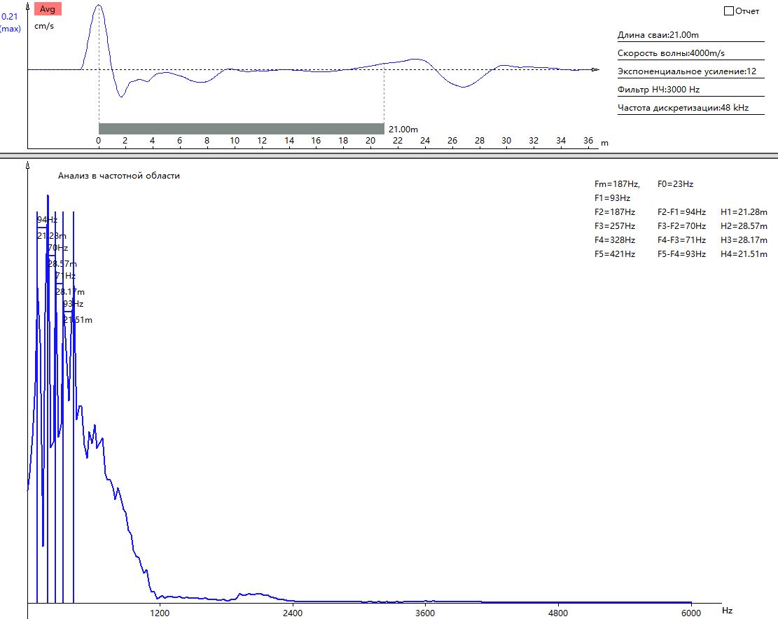
Fig. 4. Waveform and signal spectrum for a pile with a defect.
Frequency-domain analysis with the following settings: start frequency — 0 Hz; end frequency — 2400 Hz; amplitude threshold — 1; number of peaks — 5.
Let us consider a classic case of a defective pile. Look at the graphs: here the waveform and the frequency analysis agree and show the same problem.
The overall conclusion is that the pile failed the inspection. A local defect was identified in the pile shaft at a depth of about 10 metres (half its length). The wave did not reach the design toe (21 m), having reflected from an obstacle.
Fm = 187 Hz and F0 = 23 Hz do not agree: the wave reflected from a defect rather than from the toe.
The first harmonic, F1 = 93 Hz, is a reflection from a depth of 10.7 m.
H1 = 21.28 m (calculated from F2−F1 (94 Hz)) is the first multiple reflection; it indicates a depth of 10.64 m (half of 21.28 m).
The waveform peak at 21.0 m is a false peak, because frequency analysis indicates that it is not the toe but a multiple reflection from a defect located higher up.
Let us calculate the defect location using the formula:
Defect depth = V / (2 × Fdefect)
Where:
F1 = 93 Hz is the first significant frequency after the background;
V = 4000 m/s is the specified rod wave velocity for the pile;
Defect depth = 4000 / (2 × 93) ≈ 21.5 m? This agrees with H1 = 21.28 m. But this is not the depth to the defect!
In frequency analysis, F1 corresponds to a reflection from the defect rather than the toe. This means that the defect is at a depth of ≈ 10.6–10.8 m (half of 21.28 m). Why? Because the wave makes a round trip to the defect and returns. Round-trip travel time = 2L/V. Frequency = V/(2L). Hence L = V/(2F).
The refined calculation is as follows:
F = 93 Hz → L = 4000 / (2 × 93) ≈ 21.5 m — this is the round-trip path to the defect and back.
Actual defect depth = 21.5 / 2 ≈ 10.75 m.
What, then, is the waveform peak at a depth of 21.00 m?
The waveform shows the signal arrival time. If the wave reflected from a defect at 10.75 m, reached the sensor, then reflected again from the pile head and travelled downwards, it may create a false peak at a depth corresponding to a double passage (defect → head → defect → sensor). This gives an apparent depth of ~21 m.
Confirmation: in the spectrum you see F2 = 187 Hz and F3 = 257 Hz — these are harmonics that are multiples of 93 Hz (within an error). This is the classic “short-rod resonance”: the pile behaves as if it were half as long (≈10.5 m).
Let us draw a conclusion: an anomalous reflection was detected at a depth of ~10.7 m. Frequency analysis shows a dominant frequency of 93 Hz, corresponding to a shortened pile length (10.7 m). There is no reflection from the design toe (21.0 m). A defect such as a crack, void or abrupt change in cross-section is suspected at the indicated depth.
Example 3.
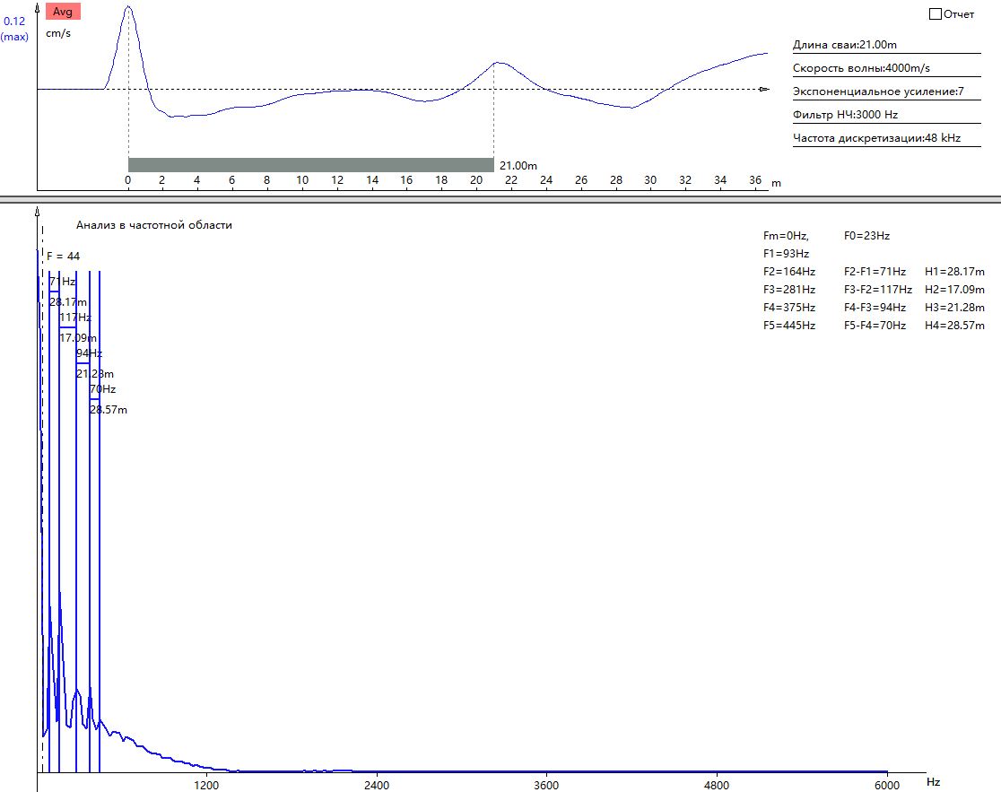
Fig. 5. Waveform and signal spectrum for a pile with a defect.
Frequency-domain analysis with the following settings: start frequency — 0 Hz; end frequency — 2400 Hz; amplitude threshold — 1; number of peaks — 5.
For this pile, the instrument cannot determine the frequency unambiguously: the signal is unstable and shows a clear spread of harmonics, which also indicates a problem.
First-approximation conclusion: the nature of the spectrum indicates a local change in cross-section or non-uniform concrete in the pile shaft. The result is unstable: this is a sign of a defect rather than interference.
F2−F1 = 117 Hz — the spacing between the 1st and 2nd harmonics corresponds to a depth of ~17.1 m (4000 / (2 × 117) ≈ 17.09 m).
F3−F2 = 94 Hz — the spacing between the 2nd and 3rd harmonics corresponds to a depth of ~21.28 m (4000 / (2 × 94) ≈ 21.28 m).
F4−F3 = 70 Hz — the spacing between the 3rd and 4th harmonics corresponds to a depth of ~28.57 m (4000 / (2 × 70) ≈ 28.57 m).
A spread from 70 Hz to 117 Hz is not normal for a defect-free pile. For a defect-free pile, all spacings should be equal to a single value (within a tolerance). Here, however, the “spacing” changes, which may be a sign of non-uniform concrete, several defects at different depths, or a varying cross-section (the pile narrows or widens).
The conclusion can be formulated as follows: frequency analysis revealed an unstable harmonic series, with spacing between harmonics varying from 70 to 117 Hz, indicating local non-uniformities in the pile shaft. The reflection from the design toe (21.00 m) on the waveform is not reliable, as it is not confirmed by a stable frequency response. The pile requires additional inspection (drilling, test-pit excavation to a depth of up to 12 m) to clarify its condition.
Analysis of a seismoacoustic signal in the spectral domain is an important component of the method for seismoacoustic testing of pile concrete integrity. With an instrument and software providing the necessary signal processing tools at hand, seismoacoustic pile testing can be performed with a high degree of reliability.
MIT KIK series instruments and software make it possible to obtain a signal of the required shape and fully analyse it for defects, even in bored piles.